Simplex Splines
Simplex splines generalize the familiar B-splines in one dimension. A k degree B-spline basis is defined for a set of k+2 points in R called knots. A B-spline basis function is a continous and smooth piecewise polynomial over R that is nonzero only over the interval bounded by the smallest and greatest knot. A set of basis functions form a space of piecewise polynomials by linear combination. In an interpolation or approximation problem, we want to choose a function from this kind of space that is the "best" in some sense. In the figure below, there are eight knots, we choose every four consecutive knots to make a quadratic B-spline basis. As an example of the interpolation problem, the coeffecients of the basis are chosen so that the linear combination (green curve) interpolates some chosen points (gray points).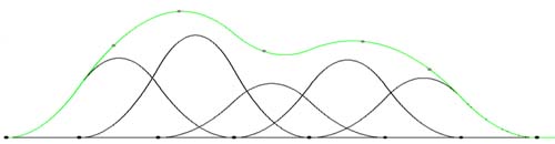 The generalization of B-spline to higher dimensions need two ingredients:
- definition of basis functions for knots in higher dimensions
- selections of knot sets given possibly irregularly-spaced knots.
 The selection of knots turns out to be quite a challenge. For 1-d B-splines, the knots are ordered and it seems "natural" to choose consecutive runs of knots as pictured earlier. Indeed, this selection yields a number of good properties. In particular, a set of degree k b-spline basis functions that arise by such a selection are proved to reproduce all polynomials of degree k. More concretely, given any degree k polynomial P, there are coeffecients for the basis set so that the linear combination using these coeffecients equals P. This polynomial-reproduction property is critical for showing some convergence properties of the spline space when used for approximation. The reproduction property implies that we can reproduce 1; this is useful if B-spline basis are used as "blending functions" of a set of curve control points.
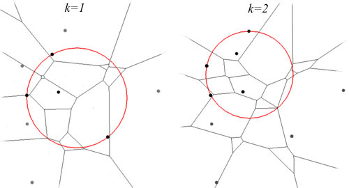
Unfortunately, in dimension greater than 1, it is not obvious how to select knot sets. Recent work of Neamtu[1] shows a way based on high order Voronoi diagrams. The selection is actually stated most concisely without reference to Voronoi: whenever we have a sphere that circumscribes s+1 knots and has k points inside, choose these k+s+1 knots as a knot set for basis construction. The centers of these spheres actually correspond to a subset of the vertices of the order k+1 Voronoi diagram, which partitions the space into cells that have the same nearest k+1 neighbors. The figure below illustrates the situation when s>=2 for varing k; each circle witnesses a knot set and is centered at a vertex of an order k+1 Vorononi diagram.
The selection of knots turns out to be quite a challenge. For 1-d B-splines, the knots are ordered and it seems "natural" to choose consecutive runs of knots as pictured earlier. Indeed, this selection yields a number of good properties. In particular, a set of degree k b-spline basis functions that arise by such a selection are proved to reproduce all polynomials of degree k. More concretely, given any degree k polynomial P, there are coeffecients for the basis set so that the linear combination using these coeffecients equals P. This polynomial-reproduction property is critical for showing some convergence properties of the spline space when used for approximation. The reproduction property implies that we can reproduce 1; this is useful if B-spline basis are used as "blending functions" of a set of curve control points.
Unfortunately, in dimension greater than 1, it is not obvious how to select knot sets. Recent work of Neamtu[1] shows a way based on high order Voronoi diagrams. The selection is actually stated most concisely without reference to Voronoi: whenever we have a sphere that circumscribes s+1 knots and has k points inside, choose these k+s+1 knots as a knot set for basis construction. The centers of these spheres actually correspond to a subset of the vertices of the order k+1 Voronoi diagram, which partitions the space into cells that have the same nearest k+1 neighbors. The figure below illustrates the situation when s>=2 for varing k; each circle witnesses a knot set and is centered at a vertex of an order k+1 Vorononi diagram.
 There are two reasons why we care about the connection to higher order Voronoi diagrams. First, for efficient computation we need to maintain Voronoi diagrams as a data structure. Second, Neamtu[1] uses some well-known geometric properties of the Voronoi diagram to prove the polynomial-reproduction property, providing a formula for reproduction that bears striking resemblance to that of the B-spline.
References and useful links
These two are from Marian Neamtu's publication page. The first one proves the reproduction of polynomials, which is the main technical result for the Voronoi-based knot set selection. The second one provides a better introduction to simplex splines and a history of the research on knot set selection.
[1] M. Neamtu, Delaunay configurations and multivariate splines: A generalization of a result of B. N. Delaunay
[2] M. Neamtu, What is the natural generalization of univariate splines to higher dimensions?, in Mathematical Methods for Curves and Surfaces
There are two reasons why we care about the connection to higher order Voronoi diagrams. First, for efficient computation we need to maintain Voronoi diagrams as a data structure. Second, Neamtu[1] uses some well-known geometric properties of the Voronoi diagram to prove the polynomial-reproduction property, providing a formula for reproduction that bears striking resemblance to that of the B-spline.
References and useful links
These two are from Marian Neamtu's publication page. The first one proves the reproduction of polynomials, which is the main technical result for the Voronoi-based knot set selection. The second one provides a better introduction to simplex splines and a history of the research on knot set selection.
[1] M. Neamtu, Delaunay configurations and multivariate splines: A generalization of a result of B. N. Delaunay
[2] M. Neamtu, What is the natural generalization of univariate splines to higher dimensions?, in Mathematical Methods for Curves and Surfaces
Higher order Voronoi diagrams (in 2D)
To compute knot sets for a degree k simplex spline, we need to compute _k+1_th order Voronoi diagrams. The size of this Voronoi diagram is at least k(n-k).Algorithms
Lee[1] is the first to give an algorithm for high order Voronoi diagrams. His approach starts out with Voronoi diagram (of order 1) and constructs successively higher order Voronoi diagrams. The basic idea is that given an i th order Voronoi Vi, the i+1 st order Voronoi Vi+1 inside a cell of Vi can be computed with local information around the cell, and the pieces of Vi+1 can then be stitched together. Lee's algorithm is static. An online algorithm is given by Boissonnat et al.[2]. Their algorithm is randomized and incremental. They maintain a graph called the Delaunay tree that is essentially the Voronoi skeletons of order one to k, together with some extra arcs that help efficient point location. The dual of a Voronoi diagram is a triangulation. In particular, it is the projection of the lower part of a polytope in 3D; the vertices of th polytope can be obtained by lifting some 2D points into 3D. Aurenhammer et al.[3]'s randomized incremental algorithm computes the dual triangulation of Voronoi this way. The main advantage of their approach is that the part of the incremental construction that maintains the connectivity is handled by 3D polytope computation, which is well studied and implemented. Also, deletion of sites is also made easy because the ``messy'' part of the computation is handled by deletion of vertices from a polytope---again a well studied and implemented computation. The asymptopic running times of the algorithms are presented below. We can see that the algorithms differ only by factors of polylog(n) or poly(k). The differences between the online algorithms are caused by point location times. Since it is well known that in practice point lcoation can be implemented most effeciently with heustics, it will be interesting to implement these algorithms without their point location routines and compare their behaviors with practical input (terrain samples points).| Lee[1] | O(k2*n*log(n)) |
| Boissonnat[2] | O(k2*n*log(n) + k*n*log3(n) ) |
| Aurenhammer[3] | O(k*(n-k)*log(n) + n*log3(n) ) |
  author =  "D. T. Lee"
, title  =   "On $k$-nearest neighbor {Voronoi} diagrams in the plane"
, journal = "IEEE Trans. Comput."
, volume =  "C-31"
, year =    1982
, pages =   "478--487"
[2] J.-D. Boissonnat and O. Devillers and M. Teillaud, A semidynamic construction of higher-order Voronoi diagrams and its randomized analysis
[3] F. Aurenhammer and O. Schwarzkopf, A simple on-line randomized incremental algorithm for computing higher order Voronoi diagrams
Software
ktess is a C++ program to compute higher order Voronoi diagram in 2D. The algorithm does the same construction as Boissonnat et al.[2] mentioned in the previous section, although the point location is done by a simple walk. The numerical computation is done with double precision floating point arithemtic so only guarantees correctness of the output with input whose precision is below 16 bits.Interpolation Problems and Ideas
Knot Selection and Fitting
We would like to use simplex splines for constructing terrain surfaces. The input will be points sampled from the terrain and the output will be a continuous and smooth surface that is the linear combination of a set of simplex spline basis functions. Assuming that we already know the set of basis functions, the unknown surface is a linear functions of the coeffcients of the basis, making it well suited for interpolating fit or least-square fit. The more difficult question is what knot sets to use. There are several goals when deciding what knots to use:- The distribution of knots should mimic the distribution of input points. That is, where the input points are dense, the knots should also be dense.
- If we try to interpolate some input points, then these points should be located near the maxima of the basis functions. Otherwise, the resulting surface will have "ripples".
Terrain surface representation
Another problem, I (Leo) am quite worried about is the high complexity of a simplex spline terrain surface. In 2D, a simplex spline basis is a piecewise polynomial where each piece is a face of the complete graph of its knots. An example of this is shown on the left of the image below for a set of five knots which define a quadratic basis. The pieces of the whole spline can be collected by taking the union of pieces for each basis. This unfortunately will give us a quite complex partitioning of the plane. At the right of the image below, the knots are positoned on a grid; the degree of the spline is two; and we see the pieces of the spline within one grid cell (of a large grid).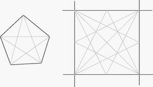 The high complexity becomes a problem if we want to represent the terrain surface as polynomial patches rather than basis + coeffcients. The former is clearly more direct and allow more effecient computation on the surface.
In comparison, other interpolation schemes not based on simplex splines explictly represent a surface as patches but have to ensure continuity and smoothness, which often involve ad-hoc methods. In other words, simplex splines avoid the continuity problem by representing the surface globally as a span of basis functions but result in a surface of high complexity. The Voronoi-based knot set selection has the promise of making things local, but it seems still not local enough. How should we resolve this?
-- YuanxinLiu - 08 Feb 2005
The high complexity becomes a problem if we want to represent the terrain surface as polynomial patches rather than basis + coeffcients. The former is clearly more direct and allow more effecient computation on the surface.
In comparison, other interpolation schemes not based on simplex splines explictly represent a surface as patches but have to ensure continuity and smoothness, which often involve ad-hoc methods. In other words, simplex splines avoid the continuity problem by representing the surface globally as a span of basis functions but result in a surface of high complexity. The Voronoi-based knot set selection has the promise of making things local, but it seems still not local enough. How should we resolve this?
-- YuanxinLiu - 08 Feb 2005
Revision: r1.1 - 28 Feb 2005 - 03:00 - Main.guest