TModeling
Start of topic | Skip to actions
Grid Filter Demo
This demo shows how to use the Grid Filter on the "Ottawa" data set
Steps 1 & 2. Build Ottawa Point Cloud Data set See the StartHere Demo.
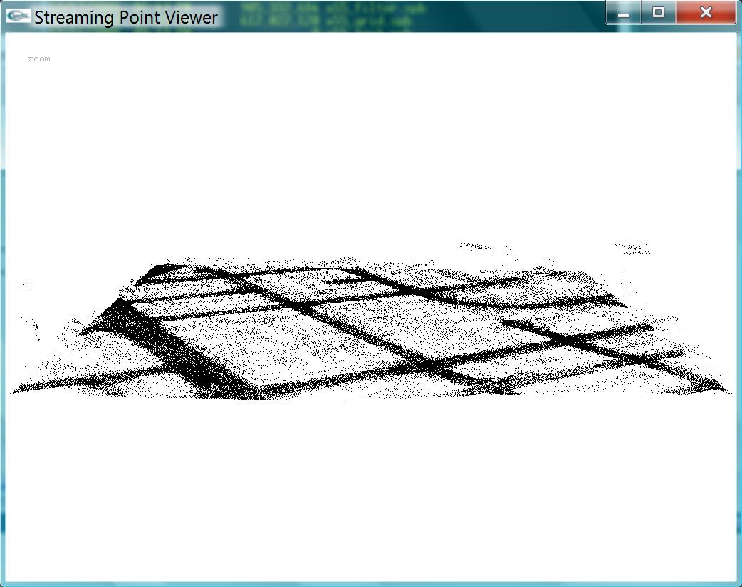
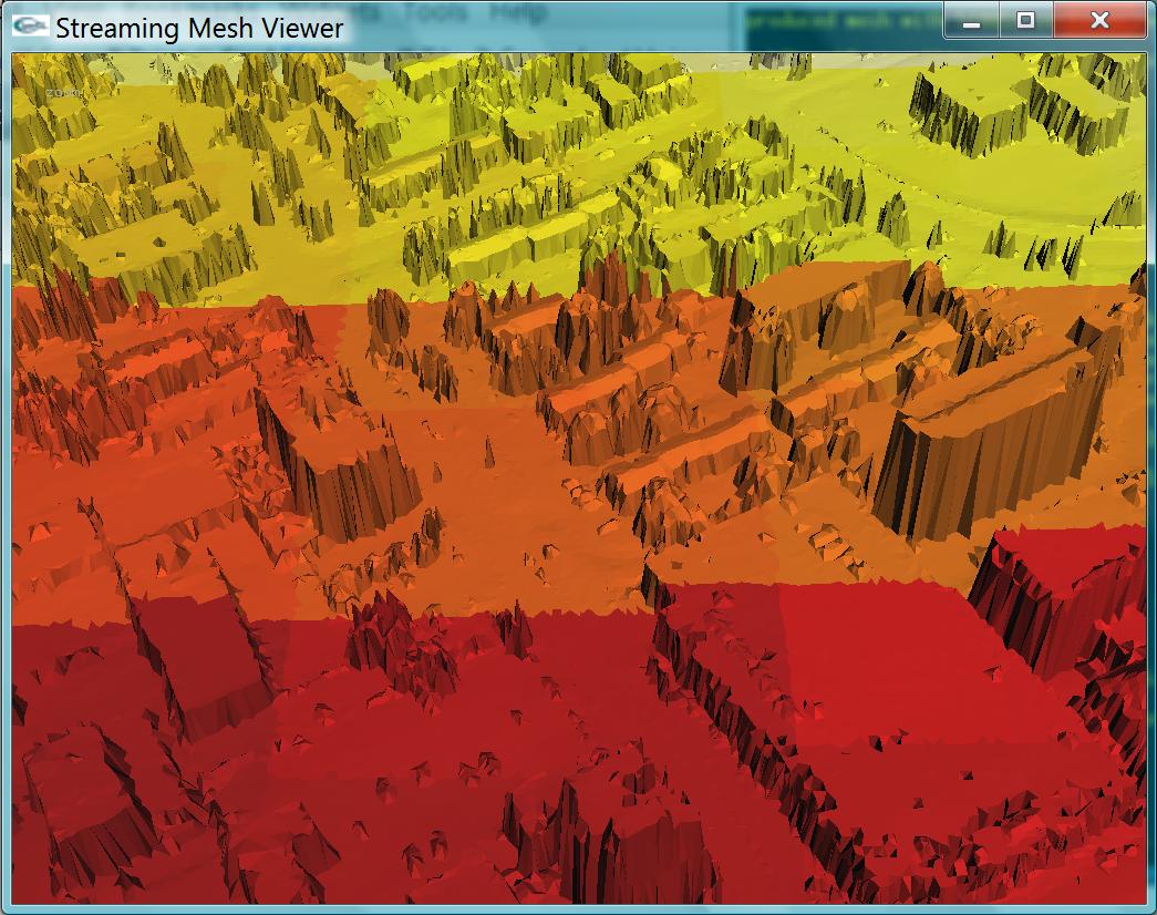
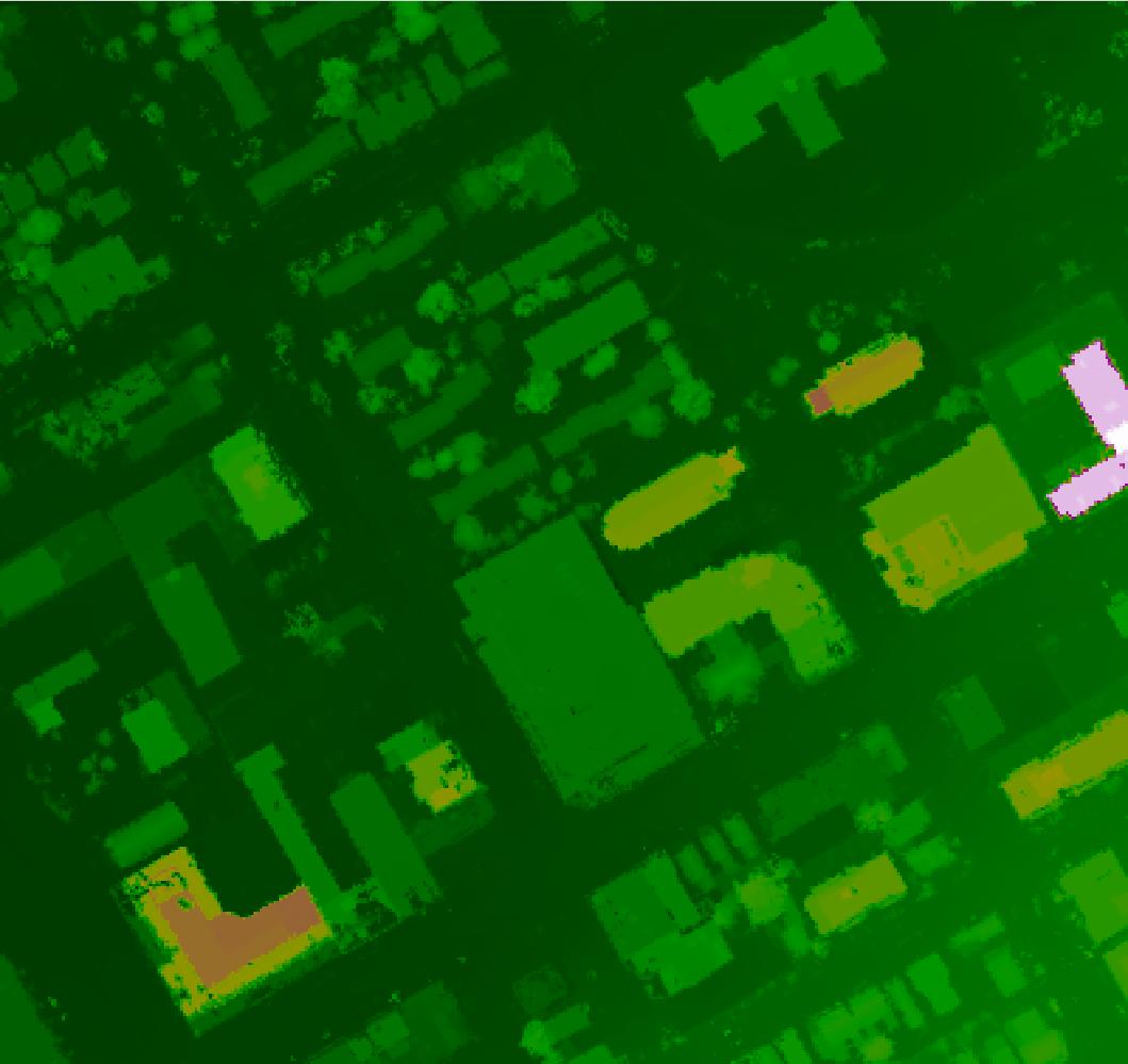
Step 3. Apply Grid Filter This step applys a grid based binning filter to the ottawa data set. Basically the point cloud is divided into a 3D grid of 1x1x1 meter^3 grid cells. then for each column we pick the grid cell containing the most points and throw away all other
points in all other grid cells in the column.
Pros:
Note: To visualize the resulting point cloud, use this command
Step 4. Spatially finalize raw point cloud data. This virtually bin's points into geographic neighborhoods using a Quad Tree Data structure. Note: This step took about 1 minutes (64 seconds) on Shawn's machine. Reading and writing to/from same disk.
Note: To visualize the resulting point cloud, use this command
Step 5. Triangulate Point Cloud Uses delaunay triangulation on the point cloud to generate a triangulated mesh. Note: Point cloud must be spatially finalized for this to work properly. Note: This step took about 3+ minutes (184.5 seconds) on Shawn's machine, reading and writing to/from same disk.
Note: To visualize the resulting mesh use the following command. This could take a very long time... I gave up part way thru
Step 6. Compress Mesh Compression is accomplished via the Quadric Error Metric (QEM), a priority heap, and edge contraction. A Quad Edge data structure is used for building the surface. Note: This step took about 28+ minutes (1681 seconds) on Shawn's Machine, reading and writing to/from same disk.
Note: To visualize the compressed mesh use the following command.
Step 7. Compress Mesh Further (Optional) Converts from .SMB format to .SMC format. Uses binary compression and the parrallelgram rule to achive an additional 2x to 10x greater compression with only a small loss in precision. Note: This step took about 3 seconds on Shawn' Machine, reading and writing to/from same disk.
Note: To visualize the compressed mesh use the following command.
Alternate Step: Remove Outliers Filter, Optional Step Filter that removes outliers. Works by computing a 1-ring neighborhood around each vertex, computing a best fit plane using linear least squares and then computing the variance of each vertex in the 1-ring to that plane. If the variance of the center point is more than 3 sigma than that point and it's incident triangles are deleted from the mesh Note: This application won't work on non-manifold mesh's. IE each vertex's 1-ring needs to have a homeomorphism to an open ball (interior vertices) or a half-ball (exterior vertices). Note: This took 14.5 seconds on Shawn's machine
Note: To visualize mesh with suppressed outlier vertices and incident triangles
 Step by Step process to regenerate mesh with fewer outliers
(and without holes caused by removing outliers)
A. Apply ring filter to remove outliers (and output to a point cloud format)
Step by Step process to regenerate mesh with fewer outliers
(and without holes caused by removing outliers)
A. Apply ring filter to remove outliers (and output to a point cloud format)
Alternate Step: Smooth Mesh, Optional Step Smooth mesh by Laplacian averaging Note: This step took about 0.7 seconds on Shawn's machine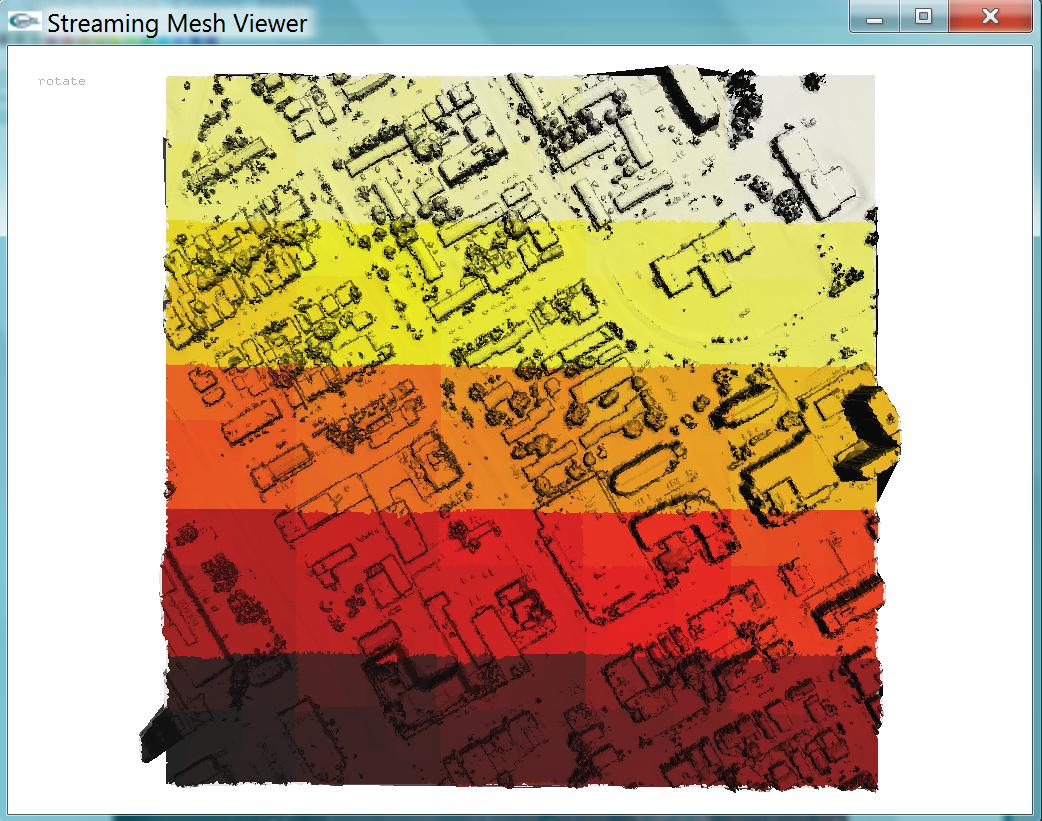
Step 8. Reorder Mesh for path finding Re-order the mesh to efficiently find a path from source to target using Dijkstra's algorithm. Note: This step took about 1.6 seconds on Shawn' Machine, reading and writing to/from same disk.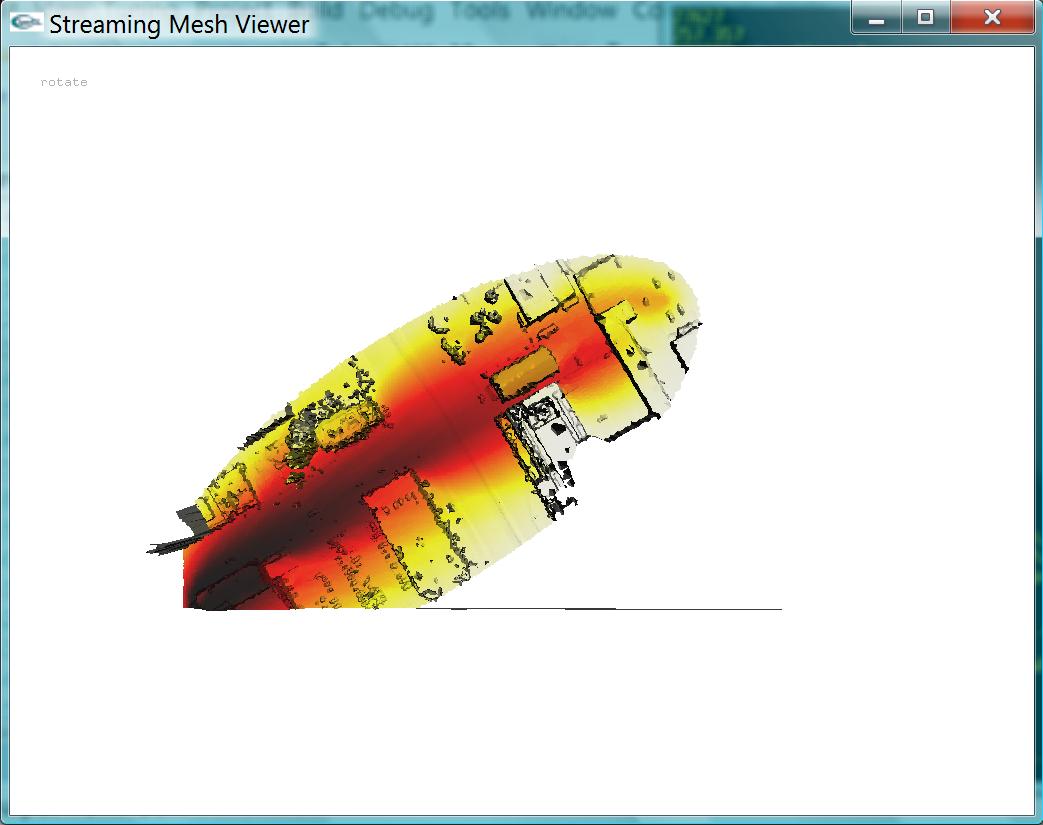
Step 9. Find Shortest Path Find shortest path using MMP algorithm. Note: This step took about 8.1 seconds on Shawn' Machine, reading and writing to/from same disk.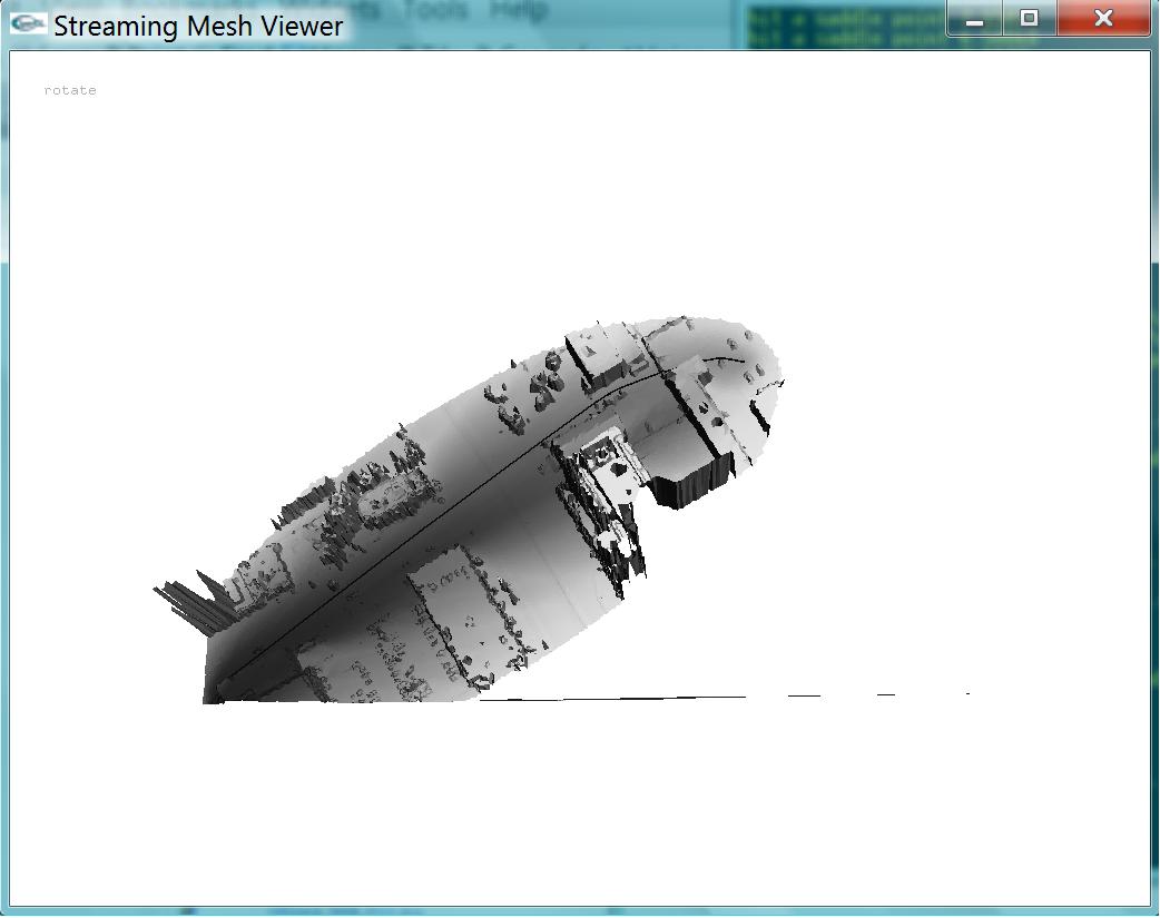
Alternate Step Rasterize TIN to DEM Converts TIN to DEM using variety of interpolation techniques (linear, matrix subdivision based on meshless wavelets, quintic, etc.) Note: This step took about 5 seconds on Shawn's Machine, reading and writing to/from same disk.
Note: To visualize the DEM you will need to use a tool like FreeView
-- ShawnDB - 18 Dec 2008
to top
This demo shows how to use the Grid Filter on the "Ottawa" data set
Steps 1 & 2. Build Ottawa Point Cloud Data set See the StartHere Demo.
Step 3. Apply Grid Filter This step applys a grid based binning filter to the ottawa data set. Basically the point cloud is divided into a 3D grid of 1x1x1 meter^3 grid cells. then for each
- The filter has the effect of picking the most important features (roads, roof-tops).
- Upside is that it tends to throw away many of the extraneous outlier points.
- It makes the data easier to delaunay triangulate as there are fewer
- Has a strong aliasing effect on the grid cell boundaries.
- Some important features get lost
spfilter -i ottawa.spb -o ottawa_grid.spb -ottawa -orig 0 0 0 -cellsize 1 1 1
| Input File: | ottawa.spb | 905 MB | 905,928,264 bytes |
| Output File: | ottawa_grid.spb | 611 MB | 611,823,464 bytes |
sp_viewer -i ottawa_grid.spb
Step 4. Spatially finalize raw point cloud data. This virtually bin's points into geographic neighborhoods using a Quad Tree Data structure. Note: This step took about 1 minutes (64 seconds) on Shawn's machine. Reading and writing to/from same disk.
spfinalize -i ottawa_grid.spb -o o55_grid.spb
| Input File: | ottawa_grid.spb | 611 MB | 611,823,464 bytes |
| Output File: | o55_grid.spb | 905 MB | 612,022,120 bytes |
sp_viewer -i ottawa55.spbNote: The resulting image is basically the same as the previous step
Step 5. Triangulate Point Cloud Uses delaunay triangulation on the point cloud to generate a triangulated mesh. Note: Point cloud must be spatially finalized for this to work properly. Note: This step took about 3+ minutes (184.5 seconds) on Shawn's machine, reading and writing to/from same disk.
spdelaunay2d.exe -i o55_grid.spb -o o55_grid_mesh.smb
| Input File: | o55_grid.spb | 905 MB | 905,332,684 bytes |
| Output File: | o55_grid_mesh.smb | 2.36 GB | 1,755,657,073 bytes |
sm_viewer -i o55_grid_mesh.smbNote: The resulting image takes too long to render, which is why it is not included here.
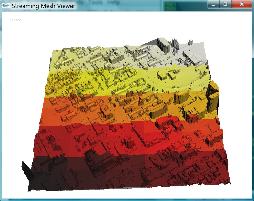
Step 6. Compress Mesh Compression is accomplished via the Quadric Error Metric (QEM), a priority heap, and edge contraction. A Quad Edge data structure is used for building the surface. Note: This step took about 28+ minutes (1681 seconds) on Shawn's Machine, reading and writing to/from same disk.
smsimpall.exe -i o55_grid_mesh.smb -o o55_grid_01.smb -buffsize 500000 -simprate 0.01 -mode 0 -retryrate 10 -zthres 135.0
| Input File: | o55_grid_mesh.smb | 1.76 GB | 1,755,657,073 bytes |
| Output File: | o55_grid_01.smb | 18.6 MB | 18,655,325 bytes |
| Original UPC file sizes 5x5 tiles | 2.77 GB | 2,773,581,424 bytes |
| Compression vs UPC | 18.6/2773 | 0.6% | 148 to 1 |
|---|---|---|---|
| Relative vs input | 18.6/1760 | 1.06% | 94 to 1 |
sm_viewer -i o55_grid_01.smb
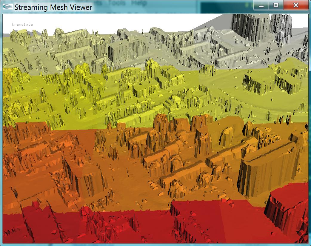
Step 7. Compress Mesh Further (Optional) Converts from .SMB format to .SMC format. Uses binary compression and the parrallelgram rule to achive an additional 2x to 10x greater compression with only a small loss in precision. Note: This step took about 3 seconds on Shawn' Machine, reading and writing to/from same disk.
sm2sm -i o55_grid_01.smb -o o55_grid_01.smc
| Input File: | o55_grid_01.smb | 18.6 MB | 18,655,325 bytes |
| Output File: | o55_grid_01.smc | 1.62 MB | 1,624,530 bytes |
| Original UPC file sizes 5x5 tiles | 2.77 GB | 2,773,581,424 bytes |
| Compression vs UPC | 1.62/2773 | 0.06% | 1707 to 1 |
|---|---|---|---|
| Relative vs input | 1.62/18.6 | 8.7% | 11.5 to 1 |
sm_viewer -i o55_grid_01.smc
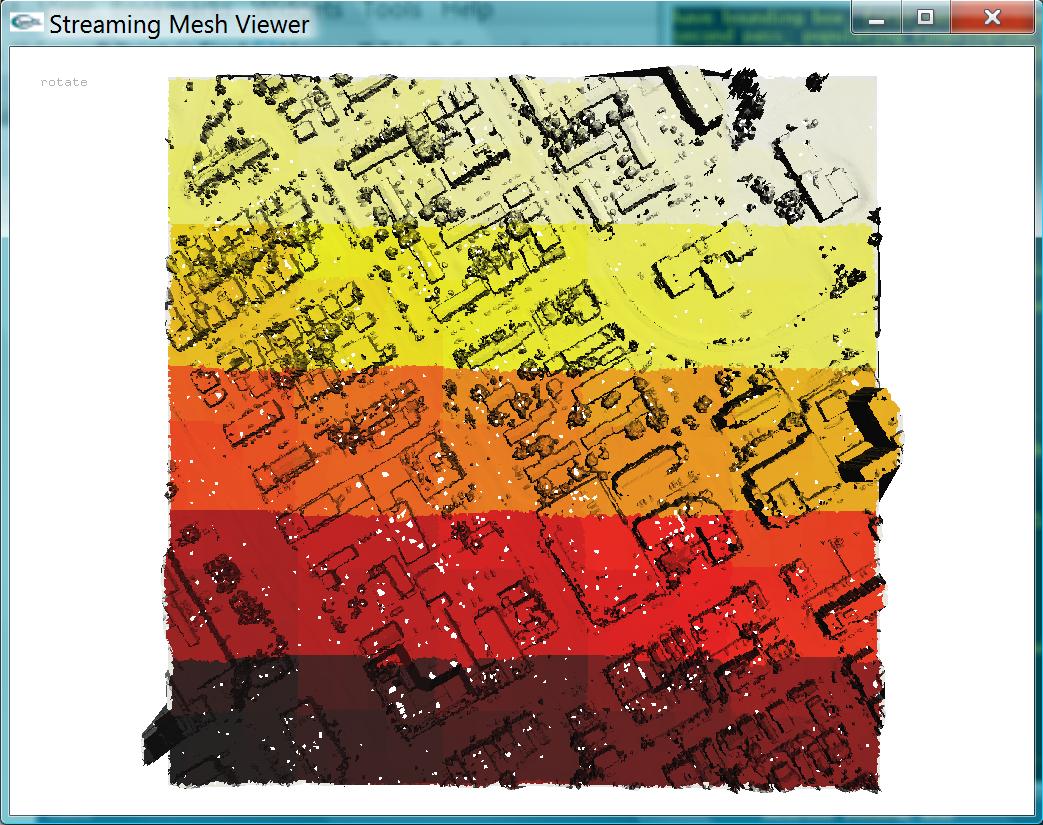
Alternate Step: Remove Outliers Filter, Optional Step Filter that removes outliers. Works by computing a 1-ring neighborhood around each vertex, computing a best fit plane using linear least squares and then computing the variance of each vertex in the 1-ring to that plane. If the variance of the center point is more than 3 sigma than that point and it's incident triangles are deleted from the mesh Note: This application won't work on non-manifold mesh's. IE each vertex's 1-ring needs to have a homeomorphism to an open ball (interior vertices) or a half-ball (exterior vertices). Note: This took 14.5 seconds on Shawn's machine
ringfilt -ismb -i o55_grid_01.smb -osmb -o o55_r2_01.smb -sigmin 0.0 -sigmax 3.0 -fl1rIn this example we suppressed...
| Suppressed Vertices | 1,850 |
| Suppressed Triangles | 9,536 |
sm_viewer -i o55_r2_01.smb
Step by Step process to regenerate mesh with fewer outliers
(and without holes caused by removing outliers)
A. Apply ring filter to remove outliers (and output to a point cloud format)
ringfilt -ismb -i o55_grid_01.smb -ospa -o o55_ring_01.spa -sigmin 0.0 -sigmax 3.0 -fl1rB. Spatially Finalize point cloud
spfinalize -i o55_ring_01.spa -o o55_ring_f_01.spbC. Turn point cloud back into a mesh by delaunauy triangulation
spdelanauy2d -i o55_ring_f_01.spb -o o55_ring_mesh_01.smbNote: To visualize the regenerated mesh with fewer outliers (spikes, etc.)
sm_viewer -i o55_ring_mesh_01.smb
Alternate Step: Smooth Mesh, Optional Step Smooth mesh by Laplacian averaging Note: This step took about 0.7 seconds on Shawn's machine
smsmooth -i o55_grid_01.smb -o o55_smooth_01.smbNote: To visualize the smoothed mesh use the following command.
sm_viewer -i o55_smooth_01.smb
Step 8. Reorder Mesh for path finding Re-order the mesh to efficiently find a path from source to target using Dijkstra's algorithm. Note: This step took about 1.6 seconds on Shawn' Machine, reading and writing to/from same disk.
dijkstra_order.exe -i o55_grid_01.smb -o grid_reorder.smb -s 1 -t 114.465027 135.945602 59.601620Note: To visualize the re-ordered mesh use the following command.
sm_viewer -i grid_reorder.smb
Step 9. Find Shortest Path Find shortest path using MMP algorithm. Note: This step took about 8.1 seconds on Shawn' Machine, reading and writing to/from same disk.
MMP.exe -i grid_reorder.smb -o grid_path.txt -s 1 -t 114.465027 135.945602 59.601620Note: To visualize the mesh and the shortest path use the following command.
sm_pathviewer -i grid_reorder.smb -path grid_path.txt
Alternate Step Rasterize TIN to DEM Converts TIN to DEM using variety of interpolation techniques (linear, matrix subdivision based on meshless wavelets, quintic, etc.) Note: This step took about 5 seconds on Shawn's Machine, reading and writing to/from same disk.
tin2dem.exe -lin -ncols 400 -nrows 400 -ulxmap 0 -ulymap 0 -xdim 1.0 -ydim 1.0 -i o55_ring_mesh_01.smb -oasc -o o55_ring_mesh_01.asc
| Input File: | o55_ring_mesh_01.smb | 18.5 MB | 18,541,265 bytes |
| Output File: | o55_ring_mesh_01.asc | 1.6 MB | 1,604,050 bytes |
-- ShawnDB - 18 Dec 2008
- Ottawa_Grid.jpg:
- Ottawa_CompGrid.jpg:
- Ottawa_Grid_SMC.jpg:
- Ottawa_Grid_RO2.jpg:
- Ottawa_Grid_Path.jpg:
- Ottawa_R2.jpg:
- Ottawa_R2_Hole.jpg:
- Ottawa_Smooth.jpg:
- Ottawa_ASC_2.jpg:
to top
| I | Attachment   | Action | Size | Date | Who | Comment |
|---|---|---|---|---|---|---|
| | Ottawa_ASC_2.jpg | manage | 72.9 K | 18 Dec 2008 - 07:44 | ShawnDB | |
| | Ottawa_CompGrid.jpg | manage | 135.1 K | 18 Dec 2008 - 03:48 | ShawnDB | |
| | Ottawa_Grid.jpg | manage | 123.0 K | 18 Dec 2008 - 03:00 | ShawnDB | |
| | Ottawa_Grid_Path.jpg | manage | 58.2 K | 18 Dec 2008 - 04:18 | ShawnDB | |
| | Ottawa_Grid_RO2.jpg | manage | 65.1 K | 18 Dec 2008 - 04:15 | ShawnDB | |
| | Ottawa_Grid_SMC.jpg | manage | 174.9 K | 18 Dec 2008 - 03:55 | ShawnDB | |
| | Ottawa_R2.jpg | manage | 157.4 K | 18 Dec 2008 - 04:52 | ShawnDB | |
| | Ottawa_R2_Hole.jpg | manage | 190.0 K | 18 Dec 2008 - 05:03 | ShawnDB | |
| | Ottawa_Smooth.jpg | manage | 164.1 K | 18 Dec 2008 - 05:11 | ShawnDB |
Edit | Attach image or document | Printable version | Raw text | More topic actions
Revisions: | r1.6 | > | r1.5 | > | r1.4 | Total page history | Backlinks
Revisions: | r1.6 | > | r1.5 | > | r1.4 | Total page history | Backlinks