Comparing shortest path methods

Overview

We will discuss the problem of finding the shortest path between two points on a terrain. Terrains can be represented in many formats. Two common terrain representations are raster representations and graph representations. Raster representations store the elevation of the terrain at regularly spaced points. Graph representations store the terrain as irregularly spaced sample points in 3D space. These sample points form the vertices of the graph; the edges are created through Delaunay triangulation. One common graph representation for terrains is a TIN (triangulated interconnect network).

The shortest path between two points is easy to find on a perfectly flat terrain with no obstructions; in this case, the shortest path is simply a straight line between the two points. In mountainous terrain, however, the shortest path between two points is not as easy to find.

When computing paths over terrain where the elevation varies, we can consider the shortest path between two points to be the path on the surface of the terrain that has the shortest distance. To do this we sample the elevation at various points, giving us points in 3D space. We then use the distance in 3D space to these sample points as our distance. This is the simplest option.

We may want to weight paths to certain points to indicate the relative difficulty of traveling between these points. We might consider going uphill harder than going downhill and assign a greater weight to an increase in eleveation than to an equal decrease in elevation. We might want to avoid steep sections, so we can use slope to place high weights on steep sections so that a shortest path will be less likely to use them. We may have routes that should not be considered, such as those that go over cliffs, and can add infinite weights to these routes.

We consider the problem of finding the shortest path in 3D space that is on the surface of the terrain. The following is a brief summary of two approaches to do so.

Sack and Lanthier

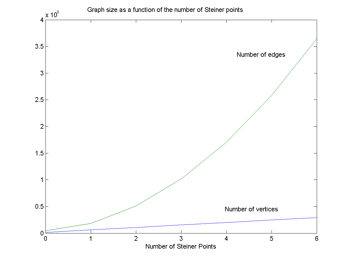
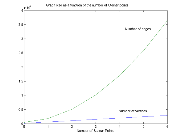
Sack and Lanthier [2] describe an approach to compute a shortest path on triangulated terrain. This approach relies on the fact that there are well-known algorithms, such as Dijkstra's algorithm, that can efficiently find the shortest path between two points in a graph. We can thus approximate the shortest path between two points in the terrain by running Dijkstra's algorithm, using these points and the terrain's graph representation as input.

To increase the accuracy of our answer, we can add more vertices and edges. We construct a graph following the approach of Sack and Lanthier. Let G be the graph from the terrain representation, and let G' be augmented graph that we construct. We add all vertices in G to G'. Between every two vertices that were connected by edges in G, we add a constant number of vertices, equally spaced. These vertices are known as Steiner points. We add an edge between each Steiner point and its neighbor, which will form a triangulated graph. We also connect each of these Steiner points to each of the other Steiner points that are on the two edges that form the opposite side of the triangle.

This process will give us a graph that we can use as input to Dijkstra's algorithm. Dijkstra's algorithm will give us the shortest path on our terrain model between the two points. The result we get becomes more accurate as we add more Steiner points to each edge. This accuracy, however, comes at the cost of a larger graph size. An analysis of the size increase is given later in this paper.

The process just described gives us a graph in which the edges have weights corresponding to distance. For this constructed graph we use linear interpolation to determine the 3D coordinates of each Steiner point and use the Euclidian distance between the two Steiner points in 3D space as the weight for the edge between the two points.

The images linked below show results from an implementation of finding shortest paths using this algorithm:

• ShortestPathSampleImages

Fast Marching

One method for computing shortest paths on a surface from raster data is to use fast marching methods. Fast marching methods track the behavior over time of a front that starts from a source point and expands outward at a positive speed. To illustrate, we will first describe the front's behavior on perfectly flat terrain and show how this behavior helps to solve our shortest paths problem. The position of the front at time 0 is our shortest paths source point. We give the front a speed of 1 meter per second. The front expands outward in a circle, and every point in the plane that the front reaches at a time of 1 second is 1 meter from the source. All plane points reached at time 2 are 2 meters away, and so on. The length of the shortest path to any point in the plane is given by the arival time.

On a raster surface we will know the elevation of the terrain at regularly spaced sample points. We will call these elevation points; between these elevation points we have a constant number of grid points. All elevation points are grid points, but not all grid points are elevation points. Since the front always expands, it passes each grid point exactly once. Each grid point has a value indicating the arrival time of the front.

We can calculate the arrival time at points on a grid using fast marching methods as follows. Kimmel and Sethian tag points as alive, near, or far [1]. Alive points are points whose arrival times have been determined, while far points are points whose arrival times have not been determined. Near points are points that have an arrival time estimated but do not have the arrival time precisely determined.

The algorithm can be summarized as follows:

• Find the near point with the smallest arrival time and mark it alive.
• Mark all neighboring points that are far as near.
• Update the arrival times of these near points based on the arrival times at neighboring alive points
• Repeat if there are still points that are not alive

We are able to mark the near point with the smallest arrival time as alive because arrival times are calculated in increasing order and are only calculated from alive points. Initially, the only points that are alive are the points that correspond to the initial position of the front. These points have an arrival time of 0. In our shortest paths problem, the front starts at a single point, so only one point is alive. We update far points adjacent to the alive points and mark them as near. We update the arrival times at near points and repeat until all points are alive.

We next describe the procedure for updating the arrival times of points based on arrival times at their alive neighbors.

Updating a grid point's arrival time based on the arrival times of its neighbors

The following figure labels the grid points surrounding the grid point to be updated. The arrival time at each grid point is indicated by the T values in the figure. In our examples, at least one of the points a, b, c, or d will be alive, and the point in the center will be near.

[1]

The following needs repair. Note that D=R*T, which you want to use as T/D = 1/R, so you actually use reciprocals of speeds... -- JackSnoeyink - 23 May 2005

Suppose that at each grid point i,j we know the front's reciprocal speed \[ F_i,j \] but not the direction; we describe how we find this speed below. We can use the front's speed and the arrival time at one or two adjacent grid points to calculate the arrival time T at grid point i,j. We assume that grid points are equally spaced at distance h. Decreasing the value of h gives us a more accurate estimates for distance at the cost of more memory.

Let p be the grid point whose arrival time we are currently updating. The method we use to update p's arrival time depends how many of p's neighbors are alive. If there is only one such neighbor a, let the front's arrival time at a be \[ T_a \]. We assume that the front moves along the horizontal or vertical line between p and a at speed \[ 1/F_i,j \]. The distance between these two grid points is the grid spacing h, so the arrival time T at p is T = Ta + h * Fi,j: (square both sides)

• 1D equation:
  [1]

If two of p's neighbors are alive and these two neighbors are not collinear with p, we follow this procedure instead. Let Ta and Tc denote the respective arrival times at adjacent points a and c. We use these arrival times in an equation whose unknown is T, the arrival time at point p.

In our problem, we know the speed of the front at point i,j. We know the arrival time of the front at grid point Ta, which is at a horizontal distance h, and the arrival time at Tc, at a vertical distance of h. The front will go a horizontal distance h in time T-Ta and a vertical distance h in time T-Tc, giving us a reciprocal velocity vector ( (T-Ta)/h, (T-Tc)/h). The length of this vector is the reciprocal of the speed of our front at point i,j. We square both sides to get the quadratic equation below.

[1]

We can ignore solutions to the quadratic equation that are before the arrival time at Ta or Tc, since we know that the front reaches a and c before it reaches p.

If arrival times at more than two grid points adjacent to the update point p are known, we follow the procedure above for every possible combination of two points where the chosen two points and p are not collinear. We set the arrival time at p to the smallest of these times. This updates the estimated arrival time for near point p.

To use this method on a terrain that is not flat we can adjust our speed function in certain places. On flat terrain the speed will still be 1, but when the terrain is not flat the speed can be slower to account for the change in elevation. One easy way to do this is to assign a cost to movement between grid points for which we have the elevation, based on the difference in elevation of these two grid points. We can adjust the speed of the front at intermediate points between these two grid points. The reciprocal of the velocity vector is _((T-Ta)/ sqrt(h^2 + (z(x,y)-z(x-h,y))^2), (T-Tc)/ sqrt(h^2 + (z(x,y)-z(x,y-h))^2))_. That just changes some of the constants in the quadratic.

Evaluating accuracy

We use DEM (digital elevation model) sample data taken from an area near Hillsborough, North Carolina. Each DEM is a 500 cell by 500 cell grid, and each cell represents an area that is 20 feet by 20 feet. The height values for cells in the grid are given in feet. We subsample the grid to make the computation faster. We choose two points in the grid, one for the source and one for the destination, and run both algorithms using the same input points. This gives us two shortest paths, one for each algorithm.

Each algorithm has a parameter that determines the tradeoff between data size and accuracy. The parameter to the Sack and Lanthier algorithm [2] will be the number of steiner points inserted on each triangle edge, while the parameter to the Kimmel and Sethian [1] algorithm will be the spacing of the grid constructed between known points.

Sack/Lanthier

We use a conversion filter to change raster data to the x,y,z points expected by the shortest paths algorithm. We connect the points according to their Delaunay triangulation. We add Steiner points along triangle edges as determined by the input parameter, and we use Dijkstra's algorithm to find the length of the shortest path between the two points.

Kimmel/Sethian

The fast marching method works on rasters, so we use the DEM raster data from the source described above. We set the grid spacing as determined by the input parameter. We start the front at the source point, and we use the arrival time at the destination point to find the length of the shortest path.

Evaluation

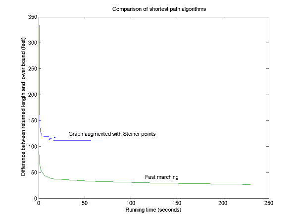
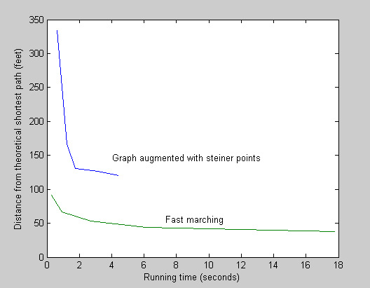
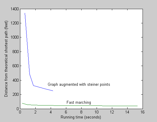
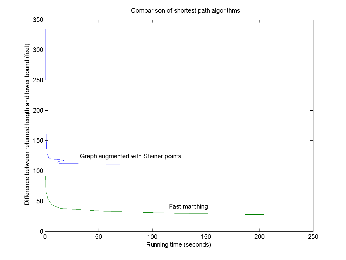
We compare shortest paths from both algorithms as a function of the accuracy parameter (number of Steiner points or grid spacing). The data will be evaluated to determine how changing these parameters affects accuracy and problem size.

Specifically, accuracy as a function of input size will be evaluated by using the number of points considered by each algorithm as the input size.

For the Sack and Lanthier algorithm, the number of points n, where v and e are the number of vertices and edges in the original graph and s is the number of steiner points added to each edge, is:

• n = v + (s * e)

For fast marching methods, let r be the number of rows and c be the number of columns in the original grid. The number of vertices v is given by v = r * c. Let h be the number of points added between two grid points. We then have

• n = (r + (h * (r - 1)) ) * (c + (h * (c - 1)) )

This works out to

• O(n) = O ( h^2 * v + 2 h * v + v ) = O(h^2 * v)

Since our implementation makes it difficult to compare input sizes, we use time as our common metric. We give results below of a run on two points. The same two points are used for both algorithms.

Results

The following results show how an implementation of Sack and Lanthier's shortest paths algorithm finds a shorter path as the number of Steiner points increases. As the number of points increases, however, so does the number of vertices and edges.

We can compare this to fast marching method results:

We can see how the difference between the returned shortest path length and the lower bound (Euclidian distance) decreases as our amount of computation time increases.

• Comparison of shortest path algorithms:
  

• More comparison:
  

• More comparison:
  

Of our two implementations, our Sack and Lanthier implementation is limited more by memory than our fast marching implementation. We ran both algorithms with the same amount of Java heap space (a maximum of 384MB), but we ran out of memory after adding 12 Steiner points to each edge. The fast marching algorithm showed a quadratic increase in time, eventually making it impractical to continue.

• ShortestPathResults -- more results (raw format)

Implementation bugs

Our fast marching algorithm occasionally returns inconsistent results, mainly around the edges of the terrain. This may have to do with our interpolation methods; the algorithm may try to interpolate based on values that lie beyond the edge of the terrain. Our results show only points between shortest paths whose returned values were consistent (the shortest path length decreased as the input size increased).

Alternate approaches

The fast marching method could be implemented by performing an 8-way update instead of a 4-way update. We take the arrival time at two adjacent grid points; in this example we have arrival times for Ta and Te.

• Figure derived from figure in [1] showing 8-way update:
  

We know the front covers a horizontal distance of h in time T-Ta, and it covers a distance of h * sqrt(2) that is half horizontal and half vertical in time T-Te. Let k = (T-Tb)/(h*sqrt(2)). We let vector F = [ T-Ta/h + (1/2)k, k ]. The length of this vector gives us the distance the front covers in one time unit, so |F|/1 = |F| is our speed at point i,j.

References

• [1] Kimmel, R. and Sethian, J. A., Computing geodesic paths on manifolds, PNAS 95:15, pp. 8431-8435, 1998.

• [2] Lanthier, M., Maheshwari, A., and Sack, J-R., Shortest Anisotropic Paths on Terrains, ICAL '99: Proceedings of the 26th International Colloquium on Automata, Languages and Programming, Springer-Verlag: London, 1999, pp. 524-533.

-- HenryMcEuen - 27 Apr 2005

to top