Ottawa Demo

Preliminaries

Goal

We were given a 5x5 set of tiles of OttawaData, consisting of 905 megabytes of point cloud data captured by NEPTEC. The data is very irregularly sampled; we show that it can be processed in this form, compressing it by a factor of 1000, and running shortest paths on the resulting surface representation.

File Formats:

We work with the following file formats for points and surfaces:

File Format	Description
.UPC	input data in format provided by NGA
.spa	Streaming Point (ASCII), human readable
.spb	Streaming Point (Binary)
.sma	Streaming mesh (ASCII), human readable
.smb	Streaming Mesh (Binary)
.smc	Streaming Mesh (Compressed Binary)

---

Test Machine Info

Our software works on 32 & 64-bit windows, Macs, and Unix. Our test machine was:

   Dell Precision WorkStation T3400
     - CPU     => Intel Core Duo (2 cores @ 3.0Ghz each)
     - Memory  => 4 GB (@ 800 Mhz)
     - OS      => Microsoft Windows XP, SP2 (64-bit)
     - Display => Nvidia Quadro FX 570
     - Drives
         C:\ => mounted on DISK0, 116+ GB capacity
         D:\ => mounted on DISK1, 232+ GB capacity
         E:\ => mounted on DISK0, 116+ GB capacity
         F:\ => mounted on CD-ROM

Step by step

1. Convert individual UPC tiles into SPB format (Point Cloud).

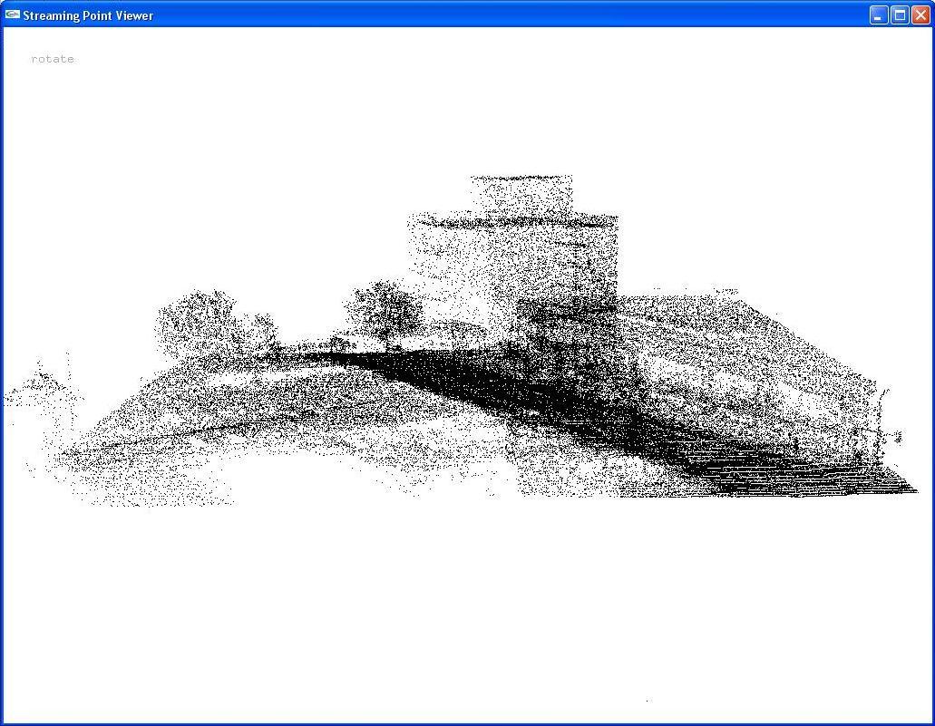
This step converts a single tile from the Ottawa Data set in UPC format into our own SPB (Streaming Point Binary) format.

Note: This step took about 2/10th's of a second. For documentation and other options, see sp2sp and sp_viewer.

   sp2sp.exe -i .\upc\000168.upc -o .\168.spb

Input File:	000168.upc	85 MB	85,440,952 bytes
Output File:	168.spb	28 MB	28,776,980 bytes

Note: To view the resulting point cloud tile, use this command

   sp_viewer.exe -i 168.spb

2. Merge all UPC Tiles into a single SPB file (Point Cloud).

Assume we have created a plain text file containing the 25 names of all the UPC files corresponding to the 5x5 square of interest named upc_files_square.txt

upc_square_files.txt

d:\OttawaDemo\upc\000147.upc
d:\OttawaDemo\upc\000148.upc
...
...
...
d:\OttawaDemo\upc\000228.upc
d:\OttawaDemo\upc\000229.upc

Then we can merge all 25 upc files into one .spb file as follows.

This step took about 48 seconds on our machine. For documentation and other options, see sp2sp

  sp2sp.exe -lof -iupc -i d:\OttawaDemo\upc_files_square.txt -ospb -o d:\OttawaDemo\ottawa.spb

We also have a suite of MATLAB scripts that can operate on all UPC files in a directory, an extract data in .rawf (raw float) formats.

Output File:

ottawa.spb

74 M pts

934 MB

934,151,264 bytes

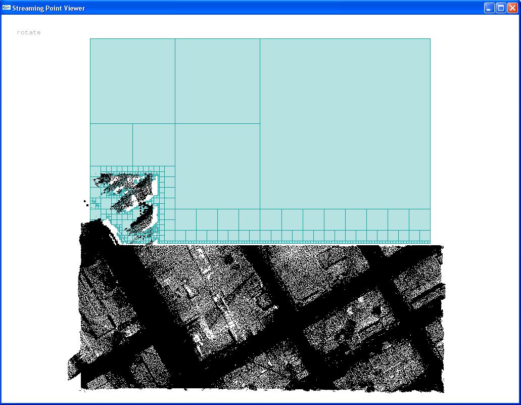
3. Spatially finalize raw point cloud data.

This virtually bin's points into geographic neighborhoods using a Quad Tree Data structure.

Note: This step took about 1/2 minutes (25 seconds) on our machine. For documentation and other options, see spfinalize and sp_viewer.

   spfinalize.exe -i ottawa.spb -o ottawa55.spb -level 8

Input File:	ottawa.spb	77 M pts	934 MB	934,151,264 bytes
Output File:	ottawa55.spb	77 M pts	937 MB	937,248,944 bytes
Memory Used:			15MB	1.7%

Note: To view the resulting point cloud, use this command

   sp_viewer.exe -i ottawa55.spb

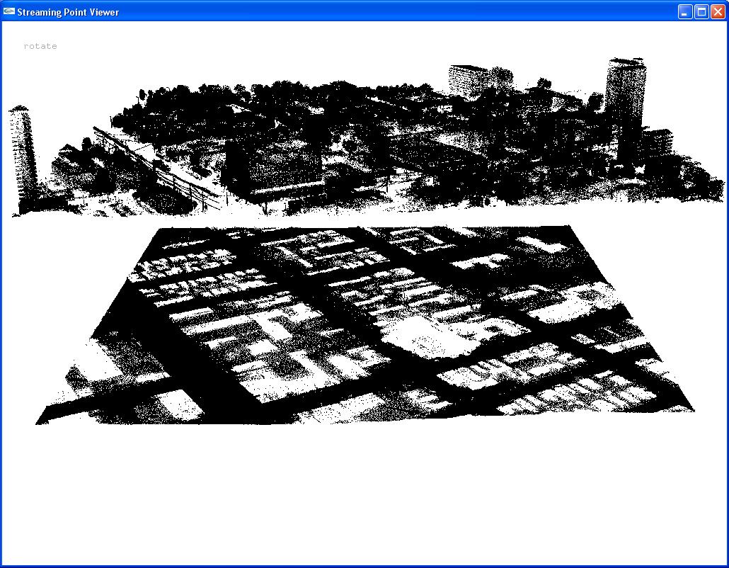
4. identify non-ground features or apply other filters.

This finds and marks non-ground features by moving their z-values above the original bounding box's max z-value. IE it essentially separates points into two groups.

   LOW - ground points (z-values remain unchanged)
   HIGH - non-ground points (z-values moved above bbox.zMax)

Note: The displayed value of zSplit can be used as the threshold by later modules to separate the two groups (LOW & HIGH)

Note: This step took about 1 1/2 minutes (83 seconds) in isolation. For documentation and other options, see spground or GridFilter.

   spground.exe -i ottawa55.spb -o o55_test.spb -tlength 30

Input File:	ottawa55.spb	77 M pts	937 MB	937,248,944 bytes
Output File:	o55_test.spb	77 M pts	937 MB	937,314,128 bytes
Memory Used:			270MB	30%
z zplit:	92.23
z sub:	163.00

Note: To view the resulting 2 layer point cloud, use this command

   sp_viewer.exe -i o55_test.spb

5. Spatially Finalize points again

The spground filter can partially destroy the spatial coherence of the original point cloud, Restore coherency by spatially finalizing the points again.

Note: This step took about 19 seconds on our machine.

   spfinalize.exe -i o55_test.spb -o o55_final.spb -level 8

Input File:	o55_test.spb	77 M pts	937 MB	937,314,128 bytes
Output File:	o55_final.spb	77 M pts	937 MB	937,248,944 bytes

Note: To view the resulting file, use this command

   sp_viewer.exe -i o55_final.spb

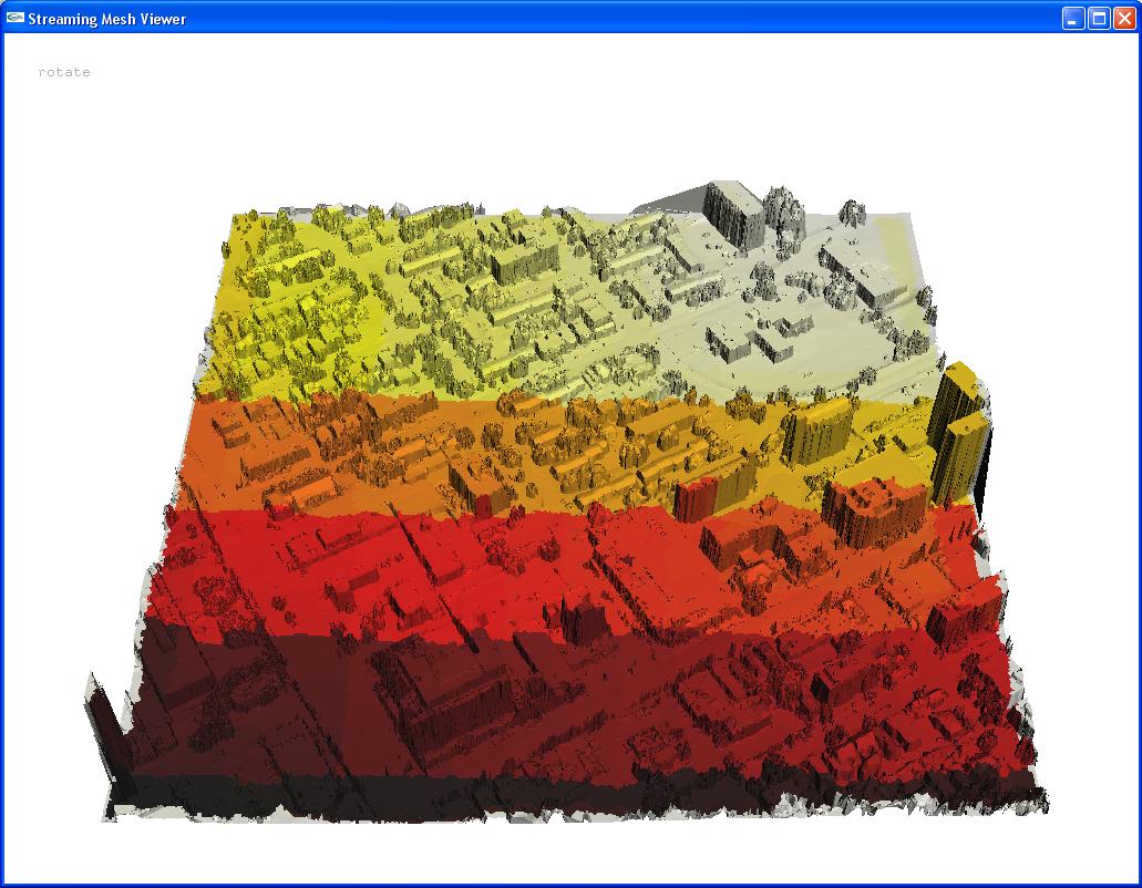
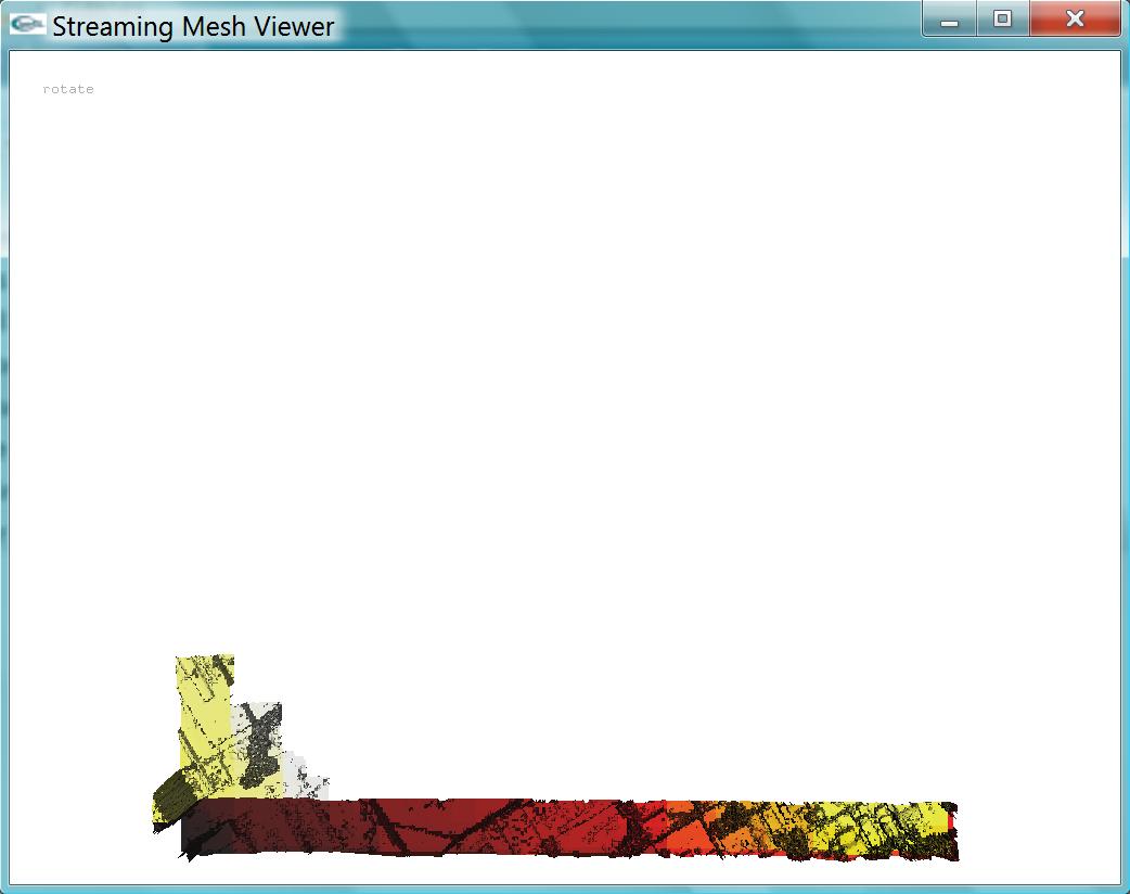
6. Triangulate Point Cloud to form TIN (Triangulated Irregular Network)

Uses Delaunay triangulation on the point cloud to generate a triangulated mesh.

Note: Point cloud must be spatially finalized for this to work properly.

Note: This step took about 2+ minutes (129.5 seconds) in isolation. For documentation and other options, see spdelaunay2d and sm_pathviewer. We recommend that the output be piped directly to simplification; there is no reason to create the large intermediate file, except for interest.

   spdelaunay2d.exe -i o55_final.spb -o o55_mesh.smb

Input File:	o55_final.spb	74 M pts	937 MB	937,248,944 bytes
Output File:	o55_mesh.smb	130 M tri	2.36 GB	2,364,655,421 bytes
Memory Used:			15MB	0.6%

Note: For smaller examples, you can view the resulting mesh use the following command. We don't recommend it with the entire 5x5 until after the next step of simplification.

   sm_pathviewer.exe -i o55_mesh.smb -zsplit 92.23 -zsub 163.0

7. Reduce Triangle Mesh

Compression is accomplished via the Quadric Error Metric (QEM), a priority heap, and edge contraction. A Quad Edge data structure is used for building the surface.

Note: This is a lossy compression technique.

Note: The code won't allow an edge contraction to occur if a triangle in the new contracted 1-ring would flip orientation from CCW to CW, IE become twisted off the manifold. This test in the 1-ring isn't sufficient to catch all potential twisting problems. Given an interior hole with a triangular ear in the current edge's 1-ring that is being tested. Any farther away vertex belonging to the same hole protruding into the ear being tested can potentially cause problems. Delta shaped interior holes are the simplest shape that can potentially cause this problem. Solving this correctly would require finding all potential problem points by walking all edges of each hole (big performance hit and may still not catch all cases in our streaming architecture), triangulating holes (including the infinite exterior face, hard to do in a streaming architecture), and/or an additional spatial location data structure (find all potential problem points in a bounding box or disc surrounding the triangle under consideration, requires covering bounding box to be spatially finalized for test to work correctly).

Note: Optionally uses a threshold value to separate points into 2 groups (LOW, HIGH) while compressing. This won't allow an edge contraction to occur if the 2 edge vertices belong to 2 different groups (HIGH & LOW). You should use the same threshold value that came from step 4.

Note: This is the time-consuming step, taking about 17.5 minutes (1051 seconds). For documentation and other options, see smsimp and sm_pathviewer.

   smsimpall.exe -i o55_mesh.smb -o o55_compress_01.smb -buffsize 500000 -simprate 0.01 -mode 0 -retryrate 10 -zthres 92.23

Original UPC:	5x5 tiles	74 M pts	2.77 GB	2,773,581,424 bytes
Input File:	o55_mesh.smb	130 M tri	2.36 GB	2,364,655,421 bytes
Output File:	o55_compress_01.smb	1.38 M tri	26 MB	26,054,753 bytes
Memory Used:			406MB	19.8%

Compression vs UPC	26/2773	0.9%	106 to 1
Compression vs input	26/2360	1.1%	91 to 1
Compression vs SPB	26/905	2.99%	36 to 1

Note: To view the simplified mesh use the following command.

   sm_pathviewer.exe -i o55_compress_01.smb -zsplit 92.23 -zsub 163.0

8. Cleanup outliers via filtering (Optional)

Uses filtering in small neighborhoods (1-rings, 2-rings) around each vertex to remove spikes and outliers.

This first filter is a planar best-fit variance filter

• For each point, get all the neighbors in it's 1-ring
• Try to fit the best plane to all the points using linear least squares
• Best fit z-val computed by substituting into resulting plane equation
• Compute the distance from the plane for the center point and it's neighbors
• Compute the variance in these distances
• Remove outliers (more than 3 sigma intervals) by replacing by the best-fit z-value

Note: This step took about 16 seconds. For documentation and other options, see RingFilt.

  ringfilt -ismb -i o55_compress_01.smb -osmb -o o55_planefit_1r.smb -sigmin 0.0 -sigmax 3.0 -fl1r -replace -zsplit 92.23 -zsub 163.0

Input File:	o55_compress_01.smb		26.0 MB	26,004,325 bytes
Output File:	o55_planefit_1r.smb	1.43 M tri	26.0 MB	25,983,953 bytes
Memory Used:			12.1MB	0.6%

Note: To view the filtered mesh use the following command.

   sm_pathviewer.exe -i o55_planefit_1r.smb -zsplit 92.23 -zsub 163.0

This Second filter is a simple height averaging variance filter

• For each point, get all the neighbors in it's 1-ring
• Compute average height (best-fit z-val)
• Compute the variance from average height for each point
• Remove outliers (more than 3 sigma intervals) by replacing by the best-fit z-value

Note: This step took about 16 seconds.

  ringfilt -ismb -i o55_planefit_1r.smb -osmb -o o55_filtered_1r.smb -sigmin 0.0 -sigmax 3.0 -f1r -replace -zsplit 92.23 -zsub 163.0

Input File:	o55_planefit_1r.smb	1.43 M tri	26.0 MB	25,983,953 bytes
Output File:	o55_filtered_1r.smb	1.43 M tri	26.0 MB	25,969,077 bytes
Memory Used:			13.6MB	0.7%

Note: To view the filtered mesh use the following command.

   sm_pathviewer.exe -i o55_filtered_1r.smb -zsplit 92.23 -zsub 163.0

Note: Note the characteristic border around the outside caused by the 3-ring state machine in RingFilt.exe

9. Storage in compressed mesh format (Optional)

Converts from .SMB format to .SMC format. Uses binary compression and the parallelogram rule to achieve an additional 10-fold compression with only a small loss in precision.

Note: This step takes about 4 seconds. For documentation and other options, see sm2sm and sm_pathviewer.

   sm2sm.exe -i o55_filtered_1r.smb -o o55_filtered_01.smc -zsplit 92.23 -zsub 163.0

Original UPC:	5x5 tiles	74 M pts	2.77 GB	2,773,581,424 bytes
Input File:	o55_compress_01.smb	1.38 M tri	25.9 MB	25,969,077 bytes
Output File:	o55_compress_01.smc	1.38 M tri	2.62 MB	2,624,364 bytes
Memory Used:			5MB	5%

Compression vs UPC	2.54/2773	0.1%	1056 to 1
Compression vs input	2.54/25.9	10.1%	9.9 to 1
Compression vs SPB	2.54/905	.28%	356 to 1

Note: To view the compressed mesh use the following command.

   sm_pathviewer.exe -i o55_filtered_01.smc

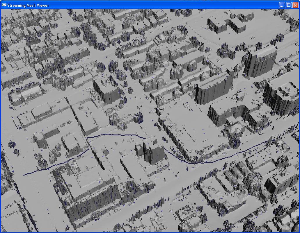
10. Find shortest path

Finds shortest path from source to destination using MMP algorithm with A* heuristic.

Note: This step took about 11 seconds on the test machine. For documentation and other options, see sm_path.

   sm_path.exe -i o55_filtered_1r.smb -s 0.0 0.0 0.0 -t 310.0 50.0 -10.0 -path path.txt 
-exact -reorder_prune out_reorder.smb 

Input File:	o55_filtered_1r.smb	25.5 MB	25,969,077 bytes
Memory Used:		312MB	1223%

Note: To view the path and reordered mesh use the following command.

   sm_pathviewer.exe -i out_reorder.smb -path path.txt -zsplit 92.23 -zsub 163.0

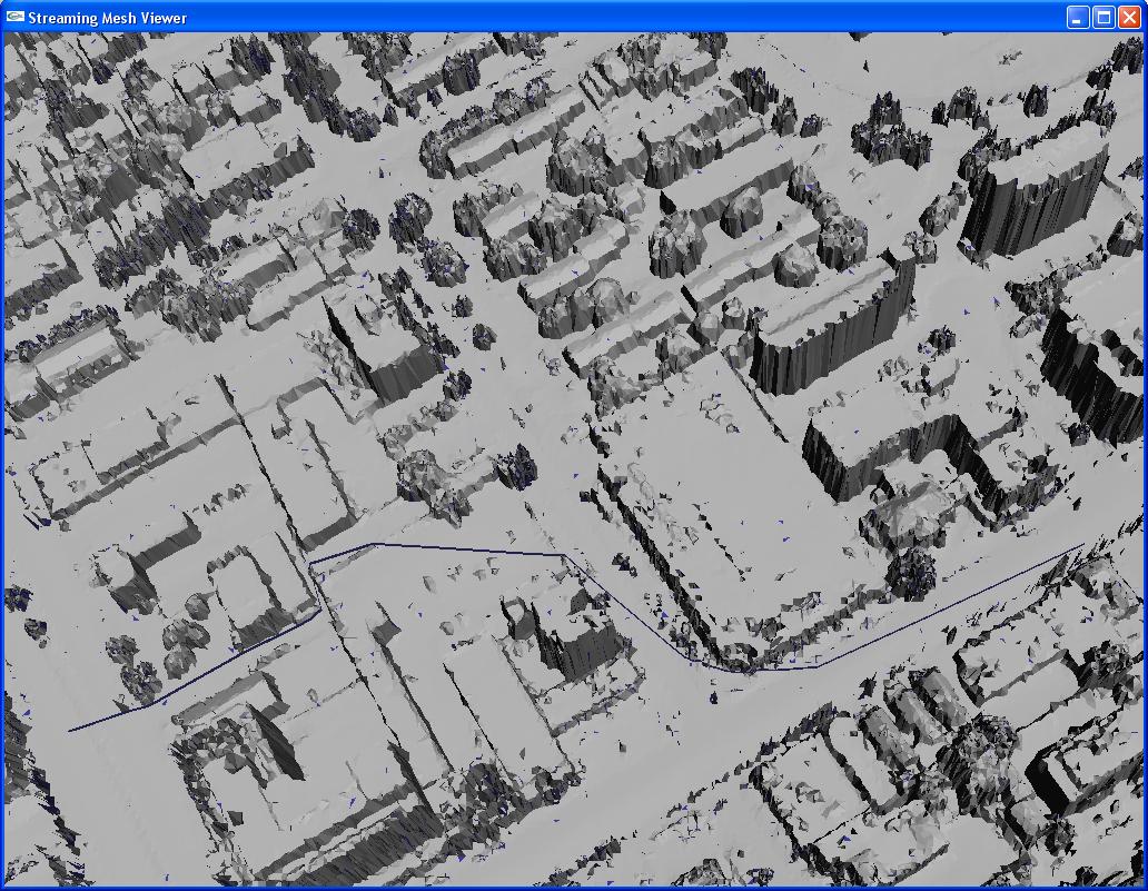Note: Here is a similar path built using Dijkstra's method. This took 1 second to compute.

Note: Notice the somewhat jagged appearance of the path caused by only allowing the path on triangle edges.

   sm_path.exe -i o55_filtered_1r.smb -s 0.0 0.0 0.0 -t 310.0 50.0 -10.0 -path dijk_path.txt 
   sm_pathviewer.exe -i out_reorder.smb -path dijk_path.txt -zsplit 92.23 -zsub 163.0

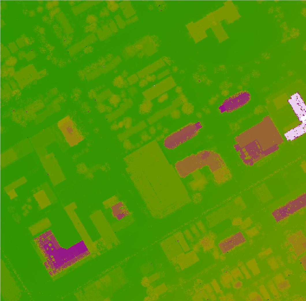
11. Rasterize TIN to DEM (Optional)

Converts TIN to DEM using variety of interpolation techniques (linear, matrix subdivision based on meshless wavelets, quintic, etc.)

Note: Can generate DEM's in ESRI ASC compatible format or .BIL format

Note: To view the DEM you will need to use a tool like FreeView or LandSerf.

Note: This step took about 1 second on the test machine, reading and writing to/from same disk.

   sm2sm.exe -i o55_compress_01.smb -osmb -zsplit 92.23 -zsub 163.0 |  tin2dem.exe -lin -ncols 400 -nrows 400 -ulxmap 0 -ulymap 0 -xdim 1.0 -ydim 1.0 -ismb -oasc -o o55_zsub_01.asc

Input File:	o55_zsub_01.smb	25 MB	25,122,013 bytes
Output File:	o55_zsub_01.asc	2.46 MB	1,603,986 bytes

---

-- ShawnDB - 16 Dec 2008

• o55_mesh.jpg:
  
• o55_reorder.jpg:
  
• Ottawa_Filt_1r.jpg:
  
• Ottawa_Square.JPG:
  
• Ottawa_Ground2.JPG:
  
• Ottawa_Compress2.JPG:
  
• Ottawa_Filter2.JPG:
  
• Path_Ontop.JPG:
  
• Path_Dijkstra.JPG:
  

to top